
31.07.2023
Page Content
Let us consider in detail measuring kilometric attenuation with a reflectometer.
OTDRs often have an automatic analysis function, but it does not always correctly determine where the dead zone is, where the FO line end is, where there is noise and, accordingly, the OTDR trace can show that the kilometric attenuation of the line is -36 dB / km, for example, which is definitely false. Therefore, it is advisable to make measurements manually.
There are two ways to do it. The first, a rougher, method is to perform it with two cursors (markers) without approximation (TPA). Just put the first cursor (marker) at the beginning of the FO line immediately after the dead zone peak, and the right – before the FO line final peak. (An orange line connecting two markers is the reference line, and when the device measures its angle of inclination, the program may conclude that there is signal loss between the markers.) Being displayed visually, as shown in the example, is an option, which can be turned on for convenience or turned off, so that not to interfere with the irregularities on the reflectometer trace).
 When setting the cursors (markers), do not touch the dead zone and the peak of the FO line end!
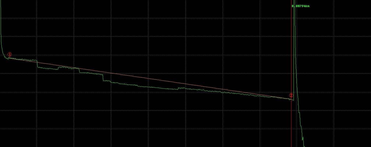
The difference in the OTDR trace values at these two points is the gross value of the line attenuation in dB. You divide it by the optical length between the cursors (markers) and get kilometric attenuation. Please note that the device itself or the computer program can make the calculation in no time and display the result. This method is rough because the reflectometer trace can be noisy, uneven and the difference in these micro-irregularities heights can reach up to a 10th decibel or more. When there is a noisy end of the long FO line it is a total catastrophe, and this method cannot be applied. This is how the OTDR trace looks like when it is strongly zoomed in (at the top right end there’s the legend of the reflectometer trace; it shows which area we zoom in and what’s the scale):
 OTDR traces noises at high zoom
For clarity, in all these examples we zoomed in the image vertically to better see where the splicing was. Without zooming, the working areas of all these OTDR traces would make almost flat lines. Also, it immediately catches your eye that the OTDR traces are noisy. The more expensive and more sensitive the OTDR device, the less noisy reflectometer traces it produces.
However, we consider a conventional reflectometer, and the FO lines are noisy, so it's better to use the second method.
The second, a more accurate method is with approximation (LSA). In this case, the program builds a virtual line that averages (approximates) all irregularities on the FO line (the least squares method is applied), and by an inclination of this line the program determines the signal loss.
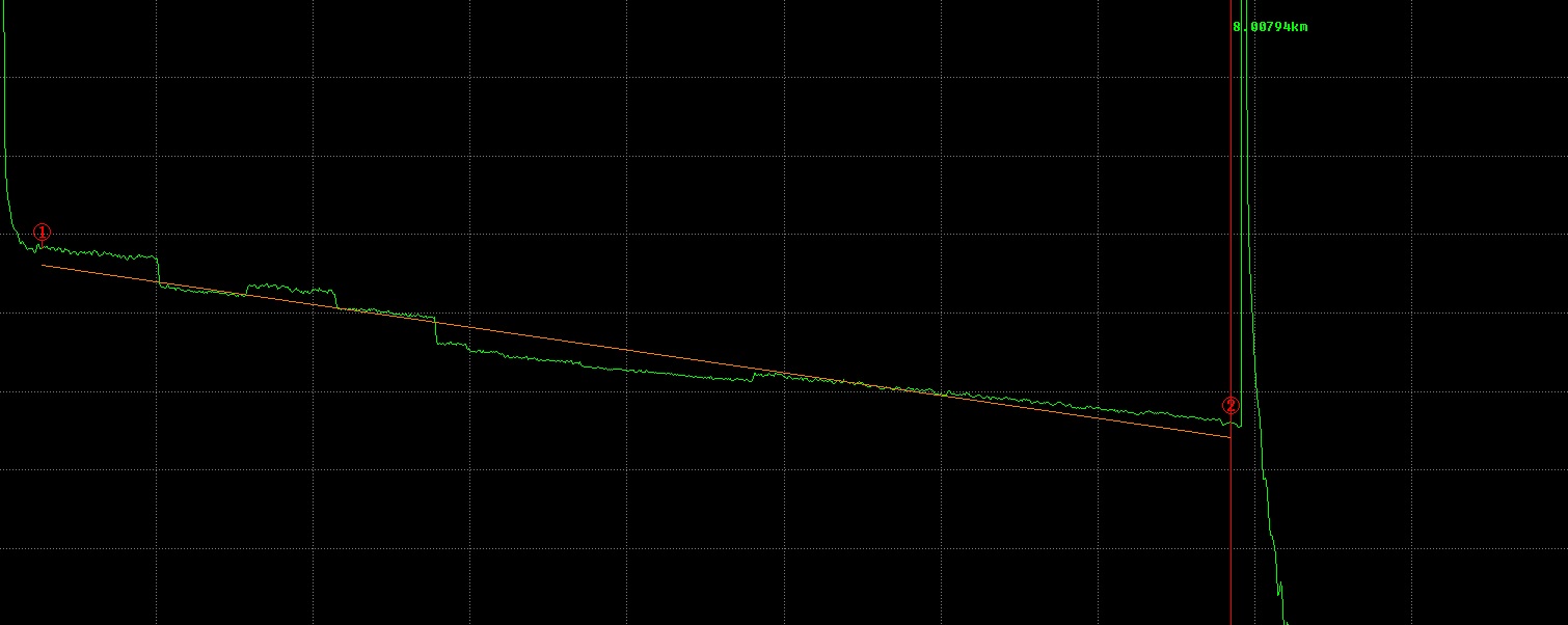
It can be seen that the reference line is no longer connected height wise with the OTDR trace where our cursors (markers) are. The reference line is calculated according to our FO line using the method of least squares. If there are many mechanical connections on the FO line with high reflection peaks, the approximation algorithm starts being approximated incorrectly and you get incorrect values. What do you do? In this case, for example, you can look at the attenuation of all the pieces of the FO line between the mechanical connections, without capturing their peaks, then separately look for the attenuation on mechanical connections (see the methods below), add up everything, and then divide by the length of the FO line. In this way you will get kilometric attenuation ... It is a long and difficult process, but if you strive for accuracy – you need to use this method.
So these nuances must be taken into account. By the way, if the FO line is very short (up to several hundred meters, when the end of the FO line comes soon after the dead zone), we cannot look at signal loss in the reflectometer trace. At this scale the OTDR trace is sometimes displayed crookedly, somewhat symbolically, and learning about attenuation is often impossible (say, it shows negative signal loss or about zero). Of course, this may depend on the device. Many inexpensive OTDRs can show this.
Now let's look at how we can observe attenuation at the irregularities point (on splice, for example).
In this case, the algorithm of actions is similar to measuring attenuation of the entire FO line, and there are also two methods: with / without approximation.
The method without approximation is simple (TPA, the method of two markers / cursors): we put the first cursor before splice, the second one immediately after it and see what signal loss we have in decibels (or, possibly, false enhancement if SM fiber is spliced with DS or NZ fiber – see above). Please remember that here only decibels are involved, and not dB / km, because splicing for us has no length. It makes no sense to talk about kilometric attenuation on splice point.
 Cursor 1 before splice point, cursor 2 – after splice point. Losses between cursors are a rough value of attenuation. The cursor here were arranged in such a way that 0.376 dB for splice point were measured. If the cursors are slightly shifted to the sides, the value will change greatly. The value of 0,376 dB on splice point is a poor result, it is necessary to fuse it again. We do not look at kilometric attenuation, because we measure the signal loss on splice point.
The method with approximation (LSA, same as the method of four markers / cursors) will be more difficult, but it also necessary to be familiar with this method and be able to use.
Here is how it looks. As we know, the OTDR trace can be noisy. So if we hit the micro-peak when placing the first cursor and we hit the micro-pit when putting the second cursor, then the device will show us a much higher signal loss on the splice point than there actually is. And vice versa, you can fail to notice poor splicing. What do we do then? The following measure will help. We take the longest possible piece of fiber without irregularities before and after splice. We construct a virtual straight line on each of these pieces (they are displayed by orange lines in the example). This will be the reflection of a flat, but noisy section of the FO line being approximated (do not forget to enable approximation using the LSA / TPA button in LSA mode). Then you can look at the level difference between the two lines in decibels.
 This method is more accurate.
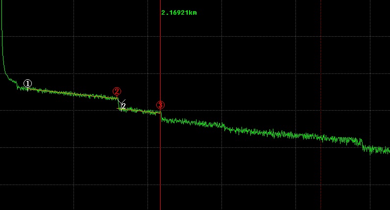
The method of four cursors is called this way because the first two markers / cursors define the boundaries of the first approximating line before splice point, and the third (in this program, for some reason, it is called Y2) and the fourth (in this program it is 3) – the second approximating line after splice point. If we arrange both lines on flat sections without irregularities, as it is done in the example (Important!), then we will learn the attenuation on splice point very accurately. Of course, this is not a final value: for conventional fusion, it is desirable, but for SM and NZ / DS splicing you just need to repeat the whole procedure on the reverse OTDR trace (from the other end of the FO line) and calculate the average value. Do this for each splice point you are interested in. And if there is no offset, no fibre core eccentricity, many specialists do not bother to make a two-sided measurement, since in this case the signal loss from A to B and from B to A will be almost the same.
We have discussed almost everything you can see on the OTDR trace. Now consider how you should configure the reflectometer for the measurement properly and how different parameters affect the performance.
To record the correct OTDR trace, you need to set the correct measurement parameters. Of course, in modern OTDRs there is an auto mode, when the required parameters are set in a hit-and-miss fashion for every new measurement. However, it is faster and more convenient to make measurements by setting parameters manually. Here again, the situation resembles a taking a photo: a beginner can take a good shot in auto mode, and a professional creates magic using manual settings. Only when it comes to an reflectometer, the main mode of operation is with manual settings, and this is faster: the OTDR will not have to "guess" how long the FO line when setting its parameters automatically.
Below is the list of important settings:
Of course, there are other settings in different devices, e.g., all kinds of settings for the clock, display, macros, but every modern person will easily figure out how to set them. There may be some specific measurement settings, in truth secondary settings, for example, a Reduced laser power: on / off setting. In this case, you need to study the instruction and think for yourself when to turn it on, and when to leave it turned off.
Let's consider how to set up the reflectometer and see the parameters effect.
It is set stepwise, for example: 300 m, 500 m, 1 km, 2 km, 5 km, 10 km, 25 km, 50 km, 100 km, etc. The smaller the minimum distance and the bigger the maximum distance an OTDR actually supports, the better the device is. It's all simple. If we roughly know how long the FO line is, we set the range a little more than twice as long as the FO line. It is twice as long so that we can see the peak of the back reflection among the noises after the FO line. It doesn’t give us a lot of information, but it is better to see this info. What if there is a broken fiber, which we can easily mistake for the end of the FO line? If we set an ample distance limit, we can probably see that the FO line continues even though there is noise. If the scale is too big, this procedure is unnecessary and undesirable: you do not want 90% of the reflectometer trace to be taken up by noise, while the FO line is at the very beginning and you cannot make out anything from the OTDR trace because of big zoom…
Important: the longer the distance you set (i.e., the measuring range), the wider the pulse and the longer the measurement time (number of averaging). This is because it takes longer for the light to travel along the long fiber, and it is more difficult for the instrument to process more data. Sometimes you really have to deal with each fiber for up to half an hour (if the FO line is more than 50 km), and still the end of the FO line is noisy. We cannot provide an exact look-up table of distance vs. pulse duration, and you need to find the best option for each measurement.
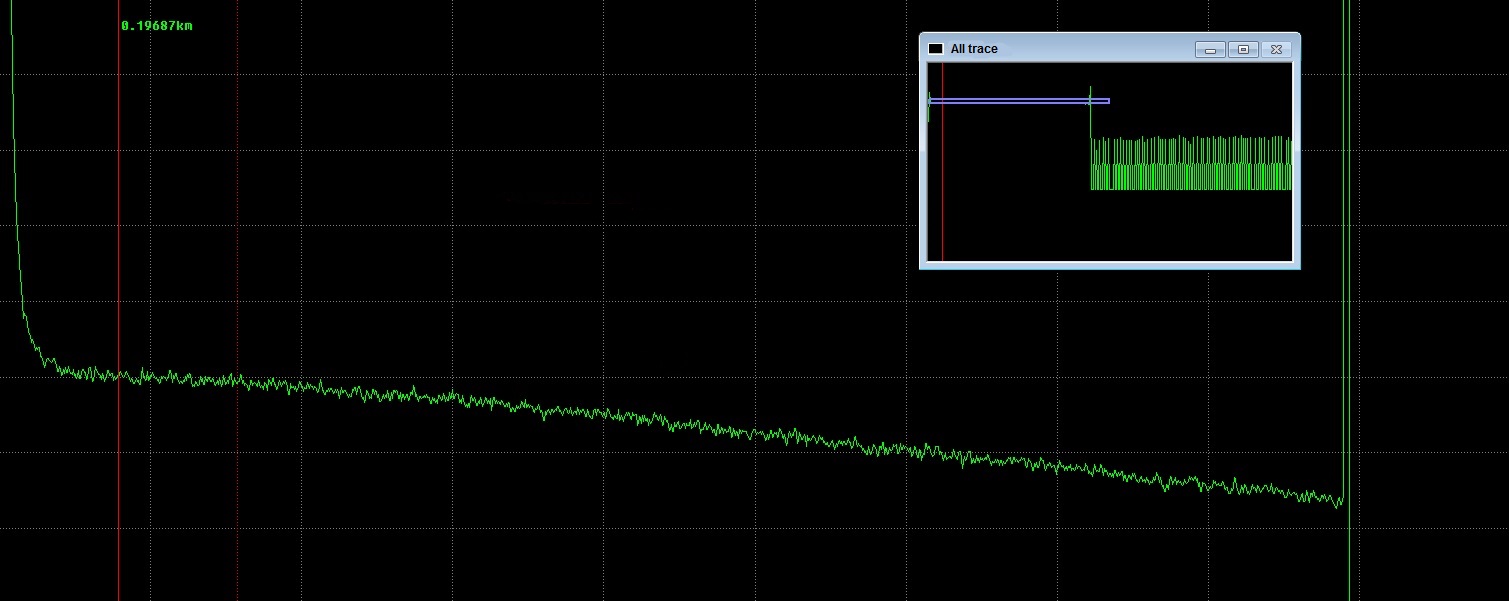
It is related to the distance you set (the bigger the range – the wider the pulse), but if necessary, the pulse duration can be changed regardless of length. Typical values range from several nanoseconds to several microseconds. For a short FO line, the pulse is short. For a long one, you need long pulse. What does the pulse length affect? Too short a pulse at a long FO line (and, correspondingly, a large distance) will cause the pulse shape to degrade severely due to the fiber dispersions, and then you will get noises. This means that we will clearly see only the beginning or the beginning + the middle of the FO line, and the end will be lost (or “drown”) in noises, like this:
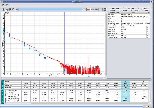 In this example, the FO line is very long, and its end is lost in noises. To see something at the end, you need to set the pulse longer and the measurement time longer too. However, if we have a cheap OTDR with a narrow dynamic range, we may never see the end of a very long FO line, even when setting an optimum impulse and measuring each fiber for an hour.
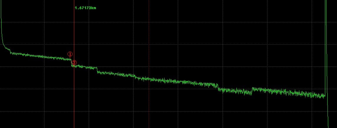
If we do the opposite, set a long pulse at a short line, it will turn out that any irregularity (the dead zone at the beginning, a "step" after each FO splice closure, a peak after each cross connect) will be strongly stretched along the Ox axis. Below is an example:
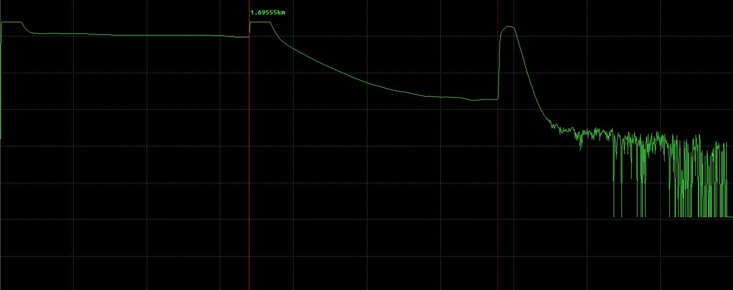
Instead of narrow signal, you see long trails. Let us explain why this happens.
Suppose you have an FO line and there was a breakdown in the middle of the line. The failure was eliminated by inserting a short-patch and two FO splice closures. If the OTDR is set correctly, even provided that the splicing was not ideal (not a model of fusion splicing) and it gives at least 0.02 dB of signal loss, and if the distance between the FO splice closures is good (about 200 m), we will clearly see two steps on the reflectometer trace, located close to each other. These steps are formed by the first and second emergency splice closures. However, if the impulse is set as too long, the trail from the first step can completely close the second splice point, and we will never know what is happening on the second splice closure!
Imagine something has happened there, for example, the water got inside, then it froze, the fibers got pinched and you need to go and make repairs urgently. Or the cable came away and it hangs bent, just about to break. The OTDR trace will simply show the trail from the first splice closure and will show that there is a signal loss somewhere. (The same situation will occur if the short-patch is short and the two FO splice closures are located side by side. Therefore, the short-patch is usually about 200 meters for long FO lines and 100 meters for short lines, otherwise we will not be able to control all splice closures in reflectometer traces, and it is very important for successful operation.)
So what impulse do we set for a particular range? There are no optimal clear look-up tables; you should try yourself, so it is necessary to understand the best conformity for your OTDR device. Again: too short a pulse on a long FO line will give excellent detail at the beginning, but the end will be lost in noise. Too long a pulse on a short FO line will lead to a loss of detail and stretching, as well as the creep in all FO line events horizontally.
The fact is that a single impulse sent to the FO line will not show us anything but noise. The laws of physics say that in order to obtain a good reflection image and to eliminate random fluctuations of Rayleigh scattering, several hundred or thousands of individual measurements should be performed, and then an average value should be taken. Thus, the more we set the number of pulses sent, the clearer and more exact our OTDR trace will be (which, in fact, is the result of approximating hundreds and thousands of individual measurements). On the other hand, there is no possibility to wait for half an hour measuring one fiber, when you need to measure 96 fibers at two wavelengths in a half-day. So you need to find a compromise.
If the FO line is long and reaches the limit of the reflectometer capacity, if the end of the FO line is subsequently noisy, then it is necessary to set a lot of averaging (about 10,000 or more) or a long measurement time (5-10 minutes), as well as a rather large pulse. On the other hand, if we check a piece of cable 300 meters long, then there is no need for super-quality, and 1000 measurements will be enough (or 10-30 seconds). By the way, in many OTDRs, it is not possible to set the number of pulses, but you can specify the measurement time in minutes / seconds. Different devices have different speed, which means that 1000 pulses can be sent by different OTDRs during different time slots; respectively, it is not reasonable to treat everyone alike and in an army fashion require the specialist to make OTDR traces, say, for 5 minutes: what if someone has an excellent fast reflectometer and 30 seconds are enough to take a perfect OTDR trace of this FO line?
Let’s make a digression here and mention such an important mode of operation as real-time mode. This means that an OTDR sends a few tens or hundreds of pulses into the FO line for about a second or two (this is not enough for a quality reflectometer trace suitable for analysis, but enough to get a general view of the FO line) and shows an average value in the OTDR trace. Then again, the OTDR sends a series of pulses and again shows the result. And it goes on until we stop it. In this case, we see what is happening on the FO line in real time at a rate of 1 image per second.
Why do we need this mode? For example, we need it to look for "crosses" and we can use this mode just to find a specific fiber. For example, we can have a following task. At the station (in the server room) there is an optical cross connect with 32 ports, a long unfamiliar FO line starts from this cross connect, and there is no documentation as usual. You need to insert a new cable into one of the FO splice closures of this FO line after 30 kilometers of the line and to splice into this cable several fibers (on cross ports 27 and 28).
How do we determine which fibers we need to cut and fuse to the new cable in that FO splice closure? Here's how we do it: we plug in the OTDR into port 27 on the cross connect and turn on the continuous mode. Once a second the FO line is shown, the image is crooked and poor, but it’s good enough to just have a look. One person works with an OTDR. Next, his partner opens the FO splice closure, telephones the person holding the OTDR and opening the cassette, gently tweezes all the fibers one by one. Of course, it is better to start with the fibers that are most likely to be ours: the fiber bend can cause a short communication break, and it will be a problem if we bend someone else's fiber.
As soon as the partner bends the fiber spliced at port 27 – the FO line seen at the reflectometer will immediately become shorter, breaking off on this splice closure point (about 30 km from the cross connect). The right fiber is immediately cut. Then fiber 28 is found in the same way, and now we know which fibers to fuse. At short distances, you can use a special flashlight (in fact a red laser pointer with an optical connector). Such a flashlight enables you to see the red light at the bending point of fibers, so no person needs to stand on the cross connect point; however, at distances beyond 5 km such laser pointer doesn’t work, besides on a bright day it is very difficult to see which fiber on the bending point shines redly – the sunshine interferes.
This factor affects the stretching of the captured OTDR trace horizontally (not to be confused with zooming in the finished OTDR trace when viewing!). The physics explanation is that in different optical fibers (for example, a conventional and offset fiber) the speed of light can be slightly different. As a result, if we measure an reflectometer trace with an incorrect refractive index, the trace will be "compressed" or "stretched" relatively to the distance gauge. This is dangerous because if there is a failure on a long FO line, we can send a team to eliminate the failure not quite where it is needed. For example, we have concluded that the break is 86 km 325 m from the cross connect and send an emergency team there. And in reality the break is through 86 km 602 m! The emergency team will be very “grateful” to us for additional 300 meters of testing under the night rain in search of where the accident happened (In fact, it can be even 900 meters! They cannot know for sure in what direction we went wrong with our conclusions).
This refractive index is an optical fiber feature and should be indicated in the cable certificate. A typical value is 1.46800, or say 1.46820.
Although for small FO lines, for example, FTTB, an error of half a meter in any direction is not so critical, and changing this coefficient all the time is inconvenient. However, on long FO lines such liberties or inaccuracies are inadmissible, this coefficient should be set exactly as it is mentioned in the cable passport; otherwise, the device can make an error +/- dozens of meters or even more. There were cases when the remedial actions were greatly delayed because of incorrect measurement.
It is necessary to make an important note. In fact, the optical cable has two lengths! The first length is the usual to us physical length, so everything is clear and simple here. It is this value that is indicated on the cable clad layer as meter marks, for example: "4000 m, 3999 m, 3998 m, ... 0 m". The second length value is optical length; in fact, this is the length of the optical fiber in the cable. It is always a bit longer than the physical length, and there is a reason for it. The cable structure usually has the modules in the cable that have lay cables. That is, for a couple of meters a sheaf of modules spins clockwise, then for couple of meters – counterclockwise, then again clockwise, etc. This is done to compensate for the changes in the length of different cable components caused by temperature changes, and also as the last, emergency protection against cable stretching: there is a chance that Kevlar, wire / fiberglass, cable cladding will break, but these lay cables will straighten out fibers or at least dampen the fiber snatching, and the fibers will survive until the emergency team arrives.
Because of this, the length of fibers (and modules) is slightly longer than the length of the cable itself. The coefficient of this layer should also be indicated in the cable certificate, although it is easy to calculate it yourself. In fact, the documentation for the FO line always indicates both the physical and optical length. Accordingly, the specialist who makes measurements should have this in mind, sending the team to the scene of the accident/failure: he will see the optical length on the OTDR trace, and the emergency team will look for the breakdown point looking at meter marks on the cable reflecting the physical length. It is bad when the FO line consists of pieces of cable of different types: for example, the buried cable is with twisted modules, and on the hang-off points, there is a cable with a single central tube-module, so in this second part, the optical length is almost equal to physical. How do we accurately determine the distance to the failure point in this case?
Here, everything is simple as well. For single-mode optical fibers, this is 1310 or 1550 nm. To prepare documentation, it is required to take OTDR traces at both wavelengths. If you do it for personal purposes (in order to better understand what is happening with the FO line), it's preferable that you record an OTDR trace at 1550 nm. At this wavelength, the attenuation is lower (we'll see the end of the FO line better), and all kinds of screwups, especially such screwups as fiber bends, are seen more clearly. By the way, if we see a poor splice on the FO splice closure, and if it shows almost the same attenuation at 1310 nm as attenuation at 1550 nm – this means the splice is really poorly fused, you need to go and fuse it again. But if at 1550 nm it is bad, and at 1310 nm it is normal or not visible at all – it most likely indicates the bend of the fiber in the cassette. You need to open the FO splice closure, the cassette and lay the cable more carefully.
In some OTDRs, you can set this parameter. Here, again, you do it similarly to setting parameters in a camera. With high resolution, we'll see irregularities better, but the OTDR trace file will be bigger, and, perhaps, the FO line will have more noises. I usually set the maximum resolution, and only if there is an unconventional situation, I start experimenting with this setting.
Another important characteristic (not setting) of the reflectometer is its dynamic range, that is, the minimum and maximum signal level an OTDR can distinguish from noise. The bigger it is, the longer the FO line we can see, the more the device will cost. When sensitivity increases, the price with grows exponentially, as always happens in such cases.
