
11.06.2018
Page Content
OTDR trace is a .sor, .trc, or other format file containing a graph with the data about the measured duct.
Attenuation is a characteristic showing how much power (dB or dBm) is lost at a given location (attenuation at splice, cross) or in a given section of the duct.
Kilometric attenuation is attenuation per unit length. If you made measurements and obtained the attenuation for the entire line of 0.66 dB and the length of your line is 3 km, then the kilometric attention will be 0.66 / 3 = 0.22 dB / km.
So, what can you read from the trace when you open it on the device or on the computer?
We will see a certain diagram. The X-axis shows the distance, the Y-axis is the signal power level. In general, the graph is descending, because everything in the fiber optic line introduces attenuation into the sent signal: all kinds of connections, defects, and the fiber itself also has constant attenuation.
An OTDR trace is made as follows: a reflectometer sends a short pulse of light (its duration is set in the settings) to the line, and then records to what is reflected back. The fiber itself, due to Rayleigh scattering, reflects back a little and analyzing the power of the reverse reflection and the time, at which this instantaneous power came, the OTDR puts dots on the axial plane, connecting them into a graph. If somewhere there is a non-reflective fault (splice, kink), then the reflectometer level of the reflected signal before the fault will be higher than after it – and a step is formed on the graph. If there is a reflective fault (mechanical connection, break, fiber end), then the OTDR trace indicates in this place a powerful reflection, much higher than the light coming from Rayleigh scattering, and we see a peak on the graph. Since the first impulse is very rough and noisy, for a quality OTDR trace, a lot of impulses (thousands and tens of thousands) are sent to the line repeatedly, and the resulting OTDR trace is their average. The more impulses, the more accurate and smooth the OTDR trace, but then you need to wait longer for the end of measurement.
The OTDR trace consists of a dead zone at the beginning, and a working area and a noise area at the end of the duct. The most typical OTDR trace is shown in the figure below:
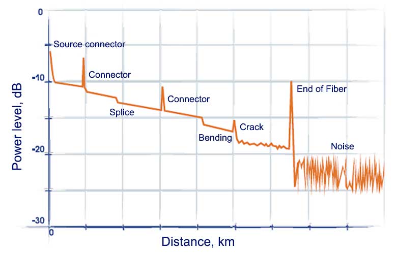
This figure will be referred to further in the text, so let us call it the "main figure".
Let us consider each element on this OTDR trace.
At the very beginning, there is a peak of the back reflection from the source connector and a loop after it - this is a so-called dead zone. The length of the duct starts from the very beginning of the reading scale, that is, the dead zone is already part of the duct we are measuring. It prevents us from seeing what happens at the very beginning of the duct, and it is sad (we cannot see directly whether the cross connection is good and whether the pigtail is well spliced with the cable).
To get rid of this dead zone completely is impossible, but you may take several measures to reduce or bypass it: you can reduce the duration of the impulse, use a more sensitive OTDR, or use a compensation coil. Yet we cannot see, say, the splice of a pigtail with a fiber of a cable in a cross, we can analyze it only from indirect data. Indirectly, one can learn about attenuation at the beginning of the duct using a compensation coil with fiber (see below).
The state of this dead zone can say a lot! The purer our mechanical connections and the ends of the patch cords / pigtails are, and the shorter we set the impulse (see below), the shorter and more accurate the dead zone will be.
If we observe that the falling edge of the dead zone forms a straight line and goes into the duct at an angle, and the dead zone is narrow (as in the figure above or on the OTDR traces from the article header), everything is set up normally.
If the same is true, but the dead zone is too wide, that means an impulse set for this duct is too long, the impulse length is too long compared to the length of our section (this is like trying to plow up the earth in a flowerpot with a conventional shovel). You need to set up a shorter impulse and measure the fiber again.
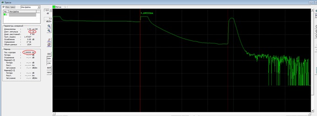
The length of the duct is very short (about 1.7 km), and the impulse is too large (1 μs). Therefore, the dead zone and all other events are stretched, "accuracy" disappears, and small details are lost. For this duct, you need to set the impulse 100 shorter. Closer to the right, there is a phantom peak at twice the distance from the end of the duct, see below for it. Moreover, more: the OTDR trace, as you can see, is "cut off" in amplitude, peaks are cut off from above. This is already a feature of an inexpensive OTDR, but this effect usually does not interfere with seeing events on the duct.
If the dead zone is not only wide, but also goes into the duct smoothly (in the form of a hyperbola / parabola), and even unevenly with noise, this is a sure sign that something is wrong at the very beginning of the duct. Either one of the ports (on the OTDR or on the cross) is dirty, or the socket on the cross or on the OTDR itself is broken. In the latter case, with repeated disconnection / connection, the result will vary greatly until complete attenuation and no sign or a signal), or the patch cord / pigtail is bad, or splice inside the cross is bad. Alternatively, the rarest and most unpleasant option, right next to the cross (tens of meters) the cable is damaged.
Another similar issue can be seen in the following cases. Sometimes, when measuring the signal at the cable hunk (or when it is necessary to measure a line not terminated with a cross connect with a cable end simply hanging), if there is no device to quick enter fibers, it is necessary to splice each fiber to the pig-tail connected to the OTDR, and after the measurement, you need to break the splice, splice another fiber, measure again, break it again, and so on.
Many operators wisely save their time and the resource of fusion splicer electrodes, tuning the fusion splicer so that it connects the fibers together, but does not give the arc (Fujikura devices allow it). At the same time, the OTDR signal goes through a small air gap and although the duct (or fiber in our checked cable hunk) is clearly visible, the dead zone also often turns out not very neat due to the air gap. It is not as terrible as in the figure below. In manual mode, looking at the fusion splicer screen, you can bring the fibers together very accurately; still, a barely noticeable axial displacement of the fibers already strongly affects the light passage through the core. The core of the fiber has a diameter of 9 μm.
Do you see the ugly the beginning of the duct? It can be worse. Most likely, it is because of a heavily dirty patch cord on the side closer to operator, but there may be a defect in the optical socket, cable damage near the cross, or bending of the fiber. If the measurement was carried out not from the cross point, but by the above-described method (when the fibers are brought together to "be measured" without splicing) - the fibers may have been poorly brought together. Thinking logically, we come to the following conclusion: if this situation is observed on all ports of the cross, then our patch cord is bad (or something is wrong with an OTDR socket, or someone was cleaning outlet sockets with a dirty cloth). If there is a single fiber like that and as a result, measurements are fluctuating for measurement to measurement after reconnecting the patch cord, then most likely a socket is defective / broken. If this is not the case, maybe he splice at cross point is poor. If there are several fibers like that and there are some that show no signal, perhaps the cable is damaged near the cross or at the exit from the base station. If the signal at 1310 nm is better than at 1550 nm, then probably there is a bend of the fiber in the cross cassette.
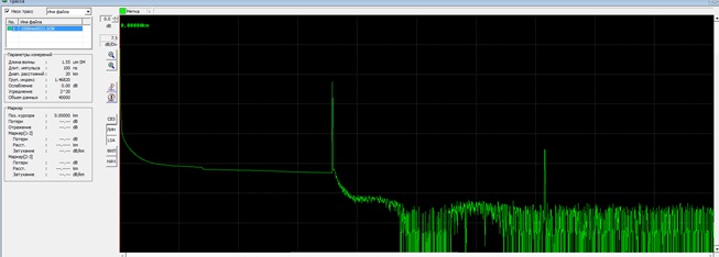
At the end of the duct, after the final peak, there is a noise area. This is no longer a duct: the duct ends with a peak before the noise. The area of noise can look different: as a series of peaks and pits, or as a flat line along the zero line, or something in between. It probably depends on the algorithm of processing and rendering the noise by the OTDR. If the back reflection at the end of the duct is strong (high peak), then a phantom peak can be detected among the noises, at a distance twice long as our duct. It can be compared figuratively to a double reflection of our face from the window glass, or the shifted contours of objects on the screen of an analog TV. The electromagnetic signal travelled through all the fiber and was reflected from the end of the duct, returned to the beginning (indicating noise and the main peak), was reflected again from the starting point of the duct, travelled again to the end of the duct, reflected again from the far end, travelled to the beginning, and only then got into the OTDR receiver (indicating noises and phantom peak among the noises). Of course, losses are great, so this phantom peak, even if it breaks through the noise, will be much weaker than the peak at the end of the route. And the events of the duct itself are never duplicated among the noises.
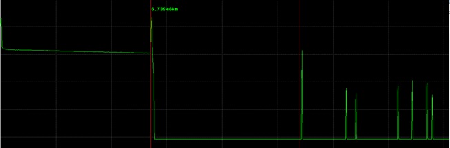
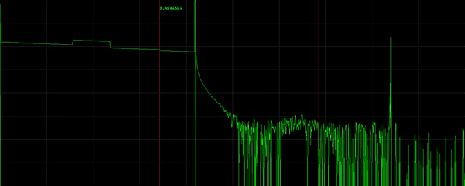
An example of a phantom peak. This duct is 6,739 km long (the red cursor is exactly at the end of the duct), and at twice the length, among the noises, we see the peak of the reverse reflection. The second pale cursor is an option in the trace program view to make sure that the given peak is a reflection, not a real event, this pale cursor, if the option is enabled, is always twice as far as the main one cursor. Pay attention to how the noise is reflected in this case: the line is at zero line and there are small "peaks".
Between the dead zone and the noise is the duct itself, our work site. In the ideal case, (we measure a single piece of cable, without splices and joints) this is a straight line. It shows a slope (gradually decreasing), since the fiber shows its own attenuation (in fiber transparency windows of single-mode fiber it is no more than 0.22 dB / km or even less at the wavelength of 1550 nm and not more than 0.36 dB / km at a wavelength of 1310 nm, and usually less, at all other wavelengths, including visible light, attenuation is much stronger). This slope is clearly visible in all pictures with examples of ducts. The shorter the duct, the less noticeable is the slope (in fact the scale of the long and short OTDR trace is different on the same screen), but the angle of inclination (with the same distance scaling) is always approximately the same and is determined by fiber attenuation.
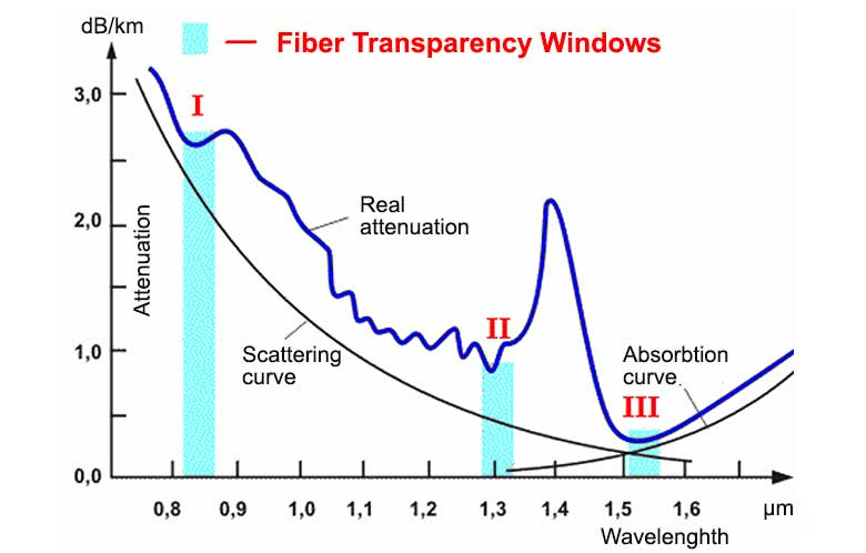
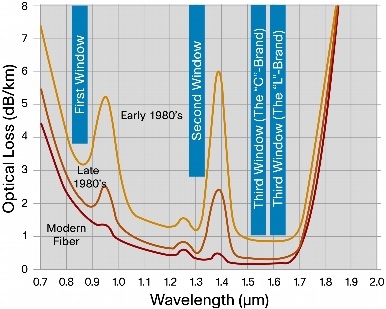
Let us make a small digression. Below is a graph (in two versions) showing the dependence of the attenuation of some optical fiber and the wavelength of the light transmitted along it. (We remember that there are a lot of fiber varieties and for each graph, it will be slightly different, this is due to the additives in the fiberglass.) On the graph, we see the working areas for our communication, the so-called transparency windows where attenuation is minimal. The first area was used before and is now of low relevance (there is high attenuation); it seems to be used in multimode fibers. The second (1310 nm) and third (1550 nm) areas are our working areas, so we chose such wavelengths (1310 and 1550 nm) so that a longer signal can be transmitted through them. For some fibers, there are other areas, with a bigger wavelength. It is clear that in each transparency window it is possible to organize many separate channels, each having its own wavelength slightly different from the neighboring one: this is how WDM (DWDM) communication systems operate.
Continued:
On an ideal duct, we will see a dead zone, a flat line (the duct itself), the end of the duct and noise. So what can we see on the working site of a real duct, between the dead zone and the end of the duct?
On some special expensive OTDRs, we can see something else: for example, the Brillouin OTDR can show where there is a dangerous mechanical stress in the fiber (for example, the sheath and Kevlar of the cable is rewound / burned and it hangs on by a thread and on some fibers, but visually it has yet been noticed). But we will not discuss these highly specialized and very expensive tools.
Let us start with the difficult one.
How can it look on the trace?
If the splice is very good and both spliced fibers are the same in properties, it may not be visible at all. With a good fusion splicer, there are a lot of such splices statistically, so it happens that in order to find a splice closure on the duct, you have to look through several traces of different fibers from this line until you get a fiber on which the splice in the splice closure is not perfect.
In most cases, splice looks like a step down. The bigger the step, the more attenuation is in this point and the poorer the splice.
How big is a step allowed? It is not such a simple question. In general, there are 2 conditions for the suitability of the duct. First, the total attenuation of the line should not exceed the above-mentioned limits (0.22 dB / km at 1550 nm and 0.36 dB / km at 1310 nm). Second, splicing with an attenuation of 0.05 dB or less is considered good, if it is more than 0.05, apparently the splicing turned out to be defective (a bubble appeared, or the axial displacement of the fibers in the fusion splicer in the point where fibers are brought together), and such splice should be fused again. If after 5 splicing attempts the attenuation does not get better, it is allowed to leave the splice with attenuation not worse than 0.1 dB.
In these two cases the result can be different. For example, we have a complex line and there are a lot of fiber closures per unit length (typical for FTTB or for sections where the cable is constantly moving from hang-out points to ground and back, respectively cable has armor or a Kevlar / wire casing interchangeably and at each transition there is a splice closure), and in this case, even if all the splices have at 0.05 dB attenuation, we may not meet the standard for kilometric attenuation! This is actually a very unpleasant situation: no one is guilty, there are no poor splices, and the customer cannot approve the object, because kilometric attenuation exceeds the norm. In this case, it is probably appropriate to ask the designing engineer why he included so many closures into the line. However, he will reply that it was the only possible option...
Or vice versa: if there are few splice closures on a long line (1 splice closure per manufactured length, and the manufactured length can be 4 and 6 km, depending on how much of cable fits into the cable drum), but on one splice closure point, the splicing brings > 0.1 dB, in general this fiber can pass the norm kilometric attenuation! Nevertheless, this splice should still be fused again.
Let us consider a more complex situation. In some cases, we can see an amazing picture: not a stepdown but a step-up! You might think that there is not attenuation at splice but the amplification of the signal. But how is this possible?
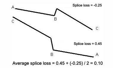
Top left: the line shows the step up first and then step down.
In fact, this increase is imaginary. When testers perform measurement, there still will be attenuation. This situation occurs when two fibers with different refractive indices and different dispersions are spliced, usually a normal SM fiber and, for example, DS or similar fiber. If we measure this splice from both sides of the line, the OTDR trace will show a step up on one side a slightly stronger step down on the other side, and the overall mean ((A + B) / 2) attenuation will still be positive. By the way, the attenuation level on one side and the imaginary attenuation rise on the other side can be quite large, up to several decibels (as in the screenshot above), although in fact the attenuation will be low in both directions.
The reason for the alleged increase is that a fiber with a displaced dispersion has a slightly different kilometric attenuation, and when another fiber enters the line section, the OTDR seemingly observes an attenuation amplification of a higher level than the actual attenuation at that splice point, and at the exit from the section it adds the same value to the attenuation at the splice point, making the splice "poor" than it is. The diagram with such step up is approximately visible in this image (different angle of the slopes of straight lines, different glass kilometer attenuation):
It is clear that in this case it is wrong to judge the quality of splicing simply by attenuation (and even more so by amplification): if on the one side the seeming increase is strong, then the seeming attenuation on the other side will be strong. When there are cable splices with different refractive indices and different dispersion, the attenuation in splice points should be determined only by measuring the line from two sides and calculating the average value. Once again, if cables with different dispersions and in general different manufacturers are fused, then it may not be the case that bad splice shown on the OTDR trace is really bad! It is necessary to measure on the other side and take the average value. (The same is true for the definition of kilometric attenuation). Strictly speaking, for conventional splices of the same fiber, you should also perform this procedure to improve accuracy, but usually it is not performed, because accuracy is sufficient and measurement is made from only one side.
Beginner operators sometimes face the following situation: they fused two different cables in the splice closure, made an OTDR trace on one side of the splice point and observe strong attenuation on some fibers. They fuse again and attenuation almost do not change. There is no change in attenuation level after next splicing either. And if we look at the situation more broadly, remembering about the possibility of seeming attenuation increase and decrease on splice points, make an OTDR standing on the other side of the line and calculate the average value for each splice (it is clear that on the reverse OTDR trace the sequence of all splices will be the mirror image of the first OTDR trace). Then everything should be normal.
Why do we have such situations in the first place? Why do we splice different fibers? It can happen when suppliers / designer engineers / storage staff made a mistake or because a cable with a part of fibers with a displaced dispersion was bought and laid in the ground, and the usual (or vice versa) cable is laid suspended (say there was no other option), and if you lay the cable again there are huge money and time losses.
The OTDR trace shows a peak, usually quite strong. It shows a peak the mechanical connection (even if this connection has angle polishing - FC / APC, SC / APC, LC / APC, or with immersion gel in the fibrlock), the reverse reflection inevitably occurs. The level of the signal after the peak usually somewhat drops, and it drops more than on the splice joint (a good connection is when it decreases 0.1 dB or less, if it decreases much more than 0.1 dB, we pick up lint-free sloth, alcohol, compressed air, cotton sticks and clean the sockets, pig-tails and patch cords, and if the fibrlock has faults we splice it again). But do not forget that with cross connect we have 1 mechanical connection and right next to it 2 fused connections! So attenuation can also cause poor splice of the cable fiber with the pigtail, and the OTDR trace does not show these 2 fusion splices and 1 mechanical connection separately, because they are too close to each other.
If the fibers with different dispersions and different kilometric attenuation are joined, the can be seeming attenuation increase as in the case of splices. What do the parameters of this peak depend on?
The stronger the reverse reflection, the higher the peak, and this is a worse situation. To reduce back reflection, patch cords and pigtails with angle polishing (FC / APC, SC / APC) are used, but usually the reflection does not cause faults in the equipment operation; this is a rare case. You can also reduce the peak height by cleaning the mechanical connection. If a very high peak is observed in the fibrlock, then you may need to replace it or just pull out the fibers, cleave them again and dip it into the immersion gel again before inserting back.
The width of the peak depends on the pulse time set on the OTDR (setting the OTDR is described next).
The signal strength before and after the peak shows how much is lost in this connection (the less the better). In long lines, mechanical connections should be avoided or at least minimized, because mechanical connection lead to a much high power loss than in fused sections (about 0.1 and 0.02, respectively).
The bending looks almost the same as splice, but with one small difference. Splice will produce approximately the same attenuation at both wavelengths. In the case of the fiber bending, the measurement at 1310 nm will not show it at all, or make it poorly visible, and at 1550 nm will produce several decibels! This is how you can understand that there is bending in the cassette, and not poor splice. If such bending appeared where there are no splice closures, it is a worrying sign that something is wrong with the cable. It is necessary to go and look, probably, the cable has been torn off the fasteners and is just damaged.
If you observe such phenomena on some splice closures, you should open the splice closures and re-lay fibers. Fibers could be displaced due to the collapse of the splice closure on the ground when someone stamped on it. And in some cases, the fibers can, over the years, fall out of the cable curving at a loop with an unacceptable bend radius in the optical cassette at the end of the module. This occurs when cables are subject to vibration and wind loads: hanging along very long bridges, along railways. Constant compression and stretching from temperature changes may add to it. The layer can slightly weaken in the modules in the cable. Why are there enough fibers to make it possible? In fact, fibers are not stretched in modules, they are laid freely, and over the years, from vibration, they can "straighten out" a little, pushing several centimeters out in both directions per 4-6 km of the manufactured length. Fibers get stronger in cables with one central module-tube, and if there are more massive cables with several modules, this effect is observed itself less.
Another reason for cable bending is when the cassette in the splice closure is designed for a 40 mm FO Splice protection kit, and 60 mm splice protection kit was crammed into it. It is clear that there is less room for maneuvers with fibers in this case, and the slightest inaccuracy and non-central laying of splice protection kits in the cradle can lead to fiber bending. Bending is a tricky case: with little inexperience, when looking at the splice closure, one cannot fail to notice that some fiber is bent too much.
Tip:
If possible, try the following: your partner is on the cross and measures the line with an OTDR continuously, and you bend fibers in the splice closure in the middle of the line, doing it more and more strongly, contacting with the partner over the phone. At a certain bend radius, he will see that peak appears on your splice closure location. Just do not overdo it, because you can break the fiber.
To feel confident with bends (and this is often necessary when dealing with problems on the line), it is advisable to practice in the following way: take a piece of the old optical cable, pull out a few fibers from it and empirically find out at which bend radius they break (both varnished and with the varnish layer removed).
It looks like a mechanical connection was applied, but the crack can lead both weaker (small peak) and much stronger peak (the peak very similar to the end of the duck, behind this huge peak at the level of noise you somehow see the duct). It is alarming when this occurred in a location where no crosses or fibrlocks are present or could be present. In fact, it happens rarely.
The line was even and smooth before it, and after it you can only record noise (sometimes among noises there’s a reflected phantom peak mentioned earlier). The end of the duct can be recorded both as a large peak and a small one; sometimes there may be no peak at all and the line breaks off immediately into noise. When having the end of the duct, we are usually not interested in how high the peak is: this is not like fusing in the middle of the duct. But if the far end of the duct is connected to the equipment and the peak is still very high, it may be necessary to clean mechanical cross connections at that end of the duct.
How do we understand that this is the end of the duct, and not a breakoff? There is only one way to do it: you need to know in advance the "regular" length of the duct. Here is an example. If we have an old OTDR trace where the duct is, say, 19.343 km long, and the new OTDR trace with the same parameters of measurement shows, say, 19.107 km and besides something does not work, you can be certain that someone was digging with an excavator on the other end of the duct :)
The rule of thumb is simple. Operators should have old OTDR traces for comparison and it is desirable to re-conduct full measurements of all fibers in your lines periodically (say, once a year), notifying clients about the scheduled outage of course. When comparing the old OTDR trace taken by constructors with the new ones, you will easily notice all problem areas, for example, fibers sticking out of the splice closure, damaged suspected, dirty sockets in the cross connect, etc. To make a comparison, you can open both OTDR traces in the program-viewer.
What about emergency communication loss? It is inconvenient to look for the old OTDF trace and “look for 10 differences” when every minute counts! For this case, operators should have a correct and up-to-date diagram of the entire line with distances indicated including the distance between splice closures (i.e., the length of cable sections) and distance from each splice closure to both ends of the duct section (up to crosses). This form is standardized and is included in the duct passport, it is form No. FOC FT-4. Operators should keep it up-to-date.
It should be said that the OTDR trace in the viewing program (and also in the device itself) can be scaled on both axes. Without scaling, the OTDR trace of a long line can look OK, with unacceptable attenuation at splice points. They are simply not visible on this screen with such resolution. If you zoom the image, all peaks will show up in all their glory. So a smooth-looking OTDR trace does not mean anything, you must always check kilometric attenuation.
How do we check kilometric attenuation of the duct? It is a very important and difficult moment. The most reliable way is to measure it with testers, or with a tester + OTDR with a tester function.
Turn on the "transmitter" mode on one tester, and the "receiver" mode on the other. Connect them with clean patch cords using a clean socket (i.e., in the following order "transmitter port - patch cord 1 - socket - patch cord 2 - receiver port").
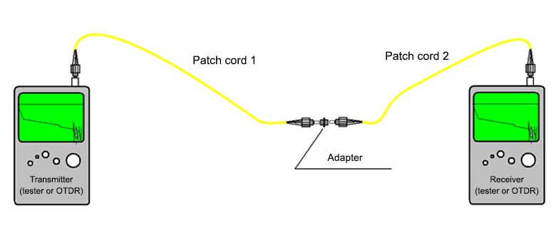
Then check what receiver tester shows. This is our "reference zero", it is even convenient to reset the receiver's readings so that this reading is the reference zero. Next, turn off the testers, disconnect the two patch cords on the socket, do not disconnect the patch cords from devices (to avoid an extra error - when the patch cord is loosened / twisted, attenuation can fluctuate from time to time!) Then carry the transmitter to one end of the duct and the receiver to the other, connect to the line and perform measurements. Remember to clean sockets in advance. A negative value (in decibels) on the receiver's display is attenuation of our entire route (if the previous value was zero, a reference zero). Divide by the optical length of our route, and you will get kilometric attenuation (dB / km). Those who love accuracy can swap devices, measure again and take the mean value as kilometric attenuation. This method is most accurate, but very uncomfortable and time-consuming. Usually, backbones are measured once a year by both testers and by an OTDR in both directions, and with ordinary (simple) lines testers are not regularly used and check just with an OTDR on one side, or even make measurement only when communication is lost. When measuring with an OTDR there are some nuances, but the overall measurement quality is quite good.
